Jupyter¶

Java logo

Grader Than Workspaces come with Jupyter installed and ready to go! In this tutorial we'll cover the basics on how to effectively teach with the immensely popular VS Code Jupyter extension which has been downloaded more than 60 million times!¹

Check out our Jupyter webinar recording.

Jupyter heavily use's markdown. It may be helpful to review our markdown tutorial before getting started. Markdown is a popular, simple, and lightweight markup language used to format text on the web.

What is Jupyter?¶

Jupyter is an open-source web application that allows you to create and share documents that contain live code, equations, visualizations, and narrative text. Jupyter notebooks are interactive documents that can be used for data analysis, machine learning, scientific computing, and more.

Jupyter notebooks support multiple programming languages, including Python, C++, Java, R, Julia, and more. This makes it a popular tool for educators that want to demonstrate code and data scientists and researchers who want to explore data, prototype algorithms, and share their work with others.

Who uses Jupyter?¶

Jupyter is used by a variety of professionals, including data educators, scientists, researchers, and developers. Some specific examples of who uses Jupyter include:

Educators: Jupyter is used in many educational settings to teach programming and data science. Jupyter notebooks can be used to create interactive tutorials and exercises, and provide a hands-on learning experience for students.
Data scientists and analysts: Jupyter is a popular tool for data analysis and exploration, and is commonly used by data scientists and analysts to prototype and test machine learning models, create visualizations, and collaborate with team members.
Researchers: Jupyter is used by researchers in many fields, including physics, astronomy, biology, and more. Researchers use Jupyter to analyze data, create visualizations, and share their results with others.
Developers: Jupyter can be used by developers to prototype and test code, create documentation, and collaborate with team members. Jupyter notebooks can also be used to create and share APIs and web applications.

How does it work?¶

Before we get our hands on the code let's briefly discuss how Jupyter works:

Jupyter provides a web-based interface for creating and editing documents called notebooks. Notebooks are organized into cells, which can contain either code or text.
When you create a new notebook, you can choose which programming language you want to use, such as Python, C++, Java, Javascript, R, Julia, or others.
Code cells in a notebook allow you to write and execute code in the notebook. When you run a code cell, the code is executed in a kernel, which is a separate process that runs on your computer.
The output of the code cell is displayed below the cell, and can include text, images, or interactive visualizations.
Markdown cells in a notebook allow you to write formatted text in the notebook using Markdown syntax. When you run a markdown cell, the text is rendered as HTML and displayed in the notebook.
Jupyter notebooks support many third-party libraries for data analysis, visualization, and machine learning, such as pandas, matplotlib, and scikit-learn.
Jupyter notebooks can be exported to a variety of file formats, including HTML, PDF, and LaTeX. This allows you to share your notebooks with others who may not have Jupyter installed.

Create a notebook¶

A notebook is a document created in Jupyter containing live code, equations, visualizations, and text in cells.

Open your Grader Than Workspace IDE
Open the command pallet in your Grader Than IDE by pressing the keys below at the same time:

Mac Linux Windows

Cmd+Shift+P

Ctrl+Shift+P

Ctrl+Shift+P
Now that the command pallet is open type > Create: New Jupyter Notebook and press Enter

This will open a new Jupyter Notebook editor that looks like the image below:

vs code jupyter notebook code cell create — This is a freshly created Jupyter Notebook

Code cells¶

In a code cell in Jupyter, you can write and execute code. The output of the code cell is displayed below the cell, which can include text, images, or interactive visualizations.

Create¶

When you create a new Jupyter Notebook in the Grader Than Workspace, a code cell will automatically be created for you. If you'd like to create another code cell press the Code button in the upper left corner of the Jupyter page. The image below references the Code button used to create a new code cell.

Run the code¶

We use Python in the following examples for example purposes. For other language specific demonstrations see the Language Specific Example section below.

Now that you've created a new code cell, write your code in the cell's text area. To run the code within an individual cell press the run button to the right of the cell.

vs code jupyter notebook run code cell — The arrow points to the button to press to run the code in the cell

Output¶

When you run a code cell the output of the code results (text, images, or GUI) will appear below the cell.

Please keep in mind the code output will be what you've printed to the console using print statements or the final unassigned functional output.

For example if you created an application that accepted keyboard input and then calculated the length of the input you'd have the following code below. When you run this code in jupyter the print statement's output and the final unassigned functional output will appear in the jupyter console.

Python Java C++

msg = input()
print(f"You typed \"{msg}\"")
len(msg)

Scanner scan = new Scanner(System.in);
String msg = scan.nextLine();
System.out.println("You typed \""+msg+"\"");
msg.length();

Where's the main() function and the import statements? See the Language specific examples section below for more details.

#include <iostream>
using namespace std;

string msg;
cin >> msg;
cout << "You typed \"" << msg << "\"";
msg.length()

Where's the main() function? See the Language specific examples section below for more details.

Input¶

When you run a code cell that requires the user to type something in, the text field to type in text will appear at the top of the screen.

Run multiple cells¶

Code cells in Jupyter are connected by a shared kernel, which allows variables and results from one cell to be used in another cell. This means that you can run code in one cell, the output or results are automatically saved, and we may then use that output or results in another cell. The shared kernel also allows you to modify and re-run code in any cell, which can update the results in other cells that depend on that code.

Running multiple code cells in Jupyter can help you break up your code into smaller, more manageable pieces, save intermediate results, and document your work.

In the example below we demonstrate how to break up our code.

vs code jupyter notebook multi code cell example — This shows an example of a multi-cell code jupyter notebook.

How did we add text?

Review this section to learn how to add text to your notebook. Additionally, read this Markdown tutorial to discover how to add text formatting, images and much more.

Notice how in the first code cell we create the variables number_1 and number_2.

First Code Cell

number_1 = 10

number_2 = 20

Then in the second code cell we define the add() function.

Second Code Cell

def add(arg_1, arg_2):
    return arg_1 + arg_2

Finally, in the last code cell, we call the add() function from the first code cell with the variables from the first code cell as arguments.

Third Code Cell

add(number_1, number_2)

This shows how we can separate our code into smaller chunks. Which make it easier to explain and demonstrate in an academic setting. Yet all the cell's runtime are connected as if they were in a single file. This means we need to run the code in the first cell before the code in the second cell.

When working with multiple code cells in Jupyter that depend on each other, it's important to run the preceding cells first before running the current code cell, to ensure that all necessary variables and functions are defined and available. Below are a few helpful buttons to run all cells above or below the given cell. You may find these buttons in the option menu that appears in the upper right corner of the selected code cell (See the image below):

vs code jupyter notebook code cell option menu — The arrow points to the code cell's option menu.

Icon	Description
	This allows you to enter a debug mode where you can run the code one line at a time and view the variable changes.
	This will run all code cells above the current code cell
	This will run all code cells below the current code cell
	This will delete the current cell.

Change a cell's language¶

By default, all Grader Than Workspace IDEs have Jupyter pre-configured to support Python and the workspace's primary programming language. If you need to switch a code cell's programming language select the language button in the bottom right corner of the code cell.

This does not change the code cell's runtime programming language. To run a particular programming language you need to change the Kernel. Read more below.

vs code jupyter notebook code cell change programming language — The arrow points to the button that allows you to change the cell's programming language.

Change the kernel¶

In Jupyter, a kernel is a separate process that runs the code in a notebook. Each notebook is associated with a particular kernel, which determines the programming language and environment for executing code in the notebook.

Changing the kernel of a notebook can be useful when you need to work with a specific version of a programming language, or when you need to use a different environment or set of libraries for your code. For example, you might switch to a kernel that includes additional libraries or packages that are not available in the default kernel.

Markdown cells¶

Markdown cells in Jupyter notebooks are cells that contain formatted text, including headings, paragraphs, lists, images, and other elements. Markdown cells use the markdown syntax, which is a lightweight markup language that allows you to add formatting to plain text. Learn more about Markdown.

Create¶

To create a markdown cell in your notebook press the Markdown button in the upper left corner of the notebook page.

Markdown cells are useful in Jupyter notebooks for providing context and documentation for your code, explaining your thought process, or providing instructions for others who may be using your notebook.

Edit¶

When the Markdown cell is in the editor mode you have the ability to type markdown or HTML in the cell's text area. When you switch the cell to preview mode the content will be rendered as HTML. To switch from edit mode to preview mode, press the check icon in the upper right corner of the cell.

Preview¶

When the markdown cell is in preview mode you will be able to view the final rendered HTML. To switch from preview mode back to the edit mode press the pencil icon in the upper right corner of the cell.

Language specific examples¶

Below are a few of our most popular language specific examples that come pre-installed in the Grader Than Workspace IDE.

Python Java C++

Jupyter was initially created in 2011 for Python. As its popularity grew, the tool was renamed to Jupyter in 2014 to support other programming languages. Python remains one of the most popular languages used in Jupyter notebooks. Today, Jupyter is widely used for education, data analysis and scientific computing.

Out of the box, almost all non-GUI standard python packages work. Because Jupyter's interface is rendered in HTML and JS there are some graphical limitations. There are several popular visualization libraries that work in Python Jupyter notebooks, including:

Matplotlib: a widely used library for creating static, animated, and interactive visualizations in Python.
IPywidgets: a way to display rich media such as images, audio, and videos in the notebook interface.
Seaborn: a library based on Matplotlib that provides a high-level interface for creating statistical graphics.
Plotly: a library for creating interactive visualizations and dashboards in Python.

Plotting GUI Turtle

The code below plots a graph that looks like a face with Matplotlib.

import matplotlib.pyplot as plt

# create the face circle
face = plt.Circle((0,0), radius=1, color='yellow')

# create the eyes
left_eye = plt.Circle((-0.3, 0.3), radius=0.1, color='black')
right_eye = plt.Circle((0.3, 0.3), radius=0.1, color='black')

# create the smile
smile = plt.Circle((0, -0.3), radius=0.4, color='black', fill=False, lw=10)

# plot the face and features
fig, ax = plt.subplots()
ax.add_artist(face)
ax.add_artist(left_eye)
ax.add_artist(right_eye)
ax.add_artist(smile)

# set the limits of the plot and remove the axis ticks
ax.set_xlim([-1.5, 1.5])
ax.set_ylim([-1.5, 1.5])
ax.set_xticks([])
ax.set_yticks([])

# show the plot
plt.show()

This demonstrates how to create a button and a button listener in a Notebook. There are many more widgets in the IPywidgets package.

from IPython.display import display
import ipywidgets as widgets


def clicked(arg):
    print("button has been clicked!")

button_download = widgets.Button(description = 'Test Button')   
button_download.on_click(clicked)
display(button_download)

Here we display an animated turtle in the notebook. We use the mobilechelonian package a modification of the popular turtle python package to render the turtle.

from mobilechelonian import Turtle
squirtle = Turtle()
squirtle.circle(50)

All Java Workspaces come with the IJava Jupyter kernel installed. This allows you to:

Write scripted code (less import statements, no class definition and no main() function)
Install maven dependencies at runtime
Display rich output, such as charts and HTML

Write scripted code

With the IJava Jupyter kernel you do not need to specify a main() function or a class this allows you to focus on the demonstrated code. Additionally, you do not need to import most standard libraries.

The code snippet below can be pasted right into Jupyter and it will automatically work.

Scanner scan = new Scanner(System.in);
String msg = scan.nextLine();
System.out.println("You typed \""+msg+"\"");
msg.length();

Install maven dependencies at runtime

With IJava you may install maven, classpath, and jar dependencies at runtime.

%%loadFromPOM
<dependency>
    <groupId>com.google.guava</groupId>
    <artifactId>guava</artifactId>
    <version>31.1-jre</version>
</dependency>

Above we use the %%loadFromPOM Cell magic to install the popular Google Guava library. Now all code cells below has access to the Google Guava library. Read more about the dependency management in IJava.

Display rich output

Jupyter's front ends provide support for display_data, and IJava interacts with the kernel's rendering API at a high level.

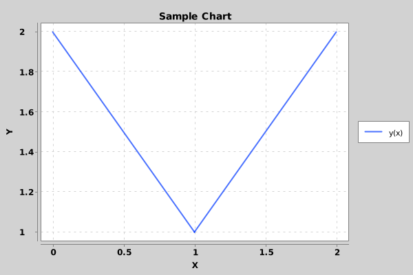
With IJava we can display charts:

%maven org.knowm.xchart:xchart:3.5.2 // (1)!

import org.knowm.xchart.*;
double[] xData = new double[] { 0.0, 1.0, 2.0 };
double[] yData = new double[] { 2.0, 1.0, 2.0 };

// Create Chart
XYChart chart = QuickChart.getChart("Sample Chart", "X", "Y", "y(x)", xData, yData);

// Display the chart
BitmapEncoder.getBufferedImage(chart);

This installs the XChart library from Maven at run time.

vs code jupyter notebook output of java xchart — This is the plot that is displayed from the code above.

We've created a simple clock that renders in HTML in the notebook. Read more below to learn about the display() and updateDisplay() functions:

import java.time.LocalDateTime;
import java.time.format.DateTimeFormatter;

String titleId = display("<h1>Clock</h1>", "text/html");
String msgId = display("", "text/html");

DateTimeFormatter formatter = DateTimeFormatter.ofPattern("HH:mm:ss");

while(true) {
    LocalDateTime now = LocalDateTime.now();
    String formattedTime = now.format(formatter);
    updateDisplay(msgId, "<b>The current time:</b> " + formattedTime, "text/html");
    Thread.sleep(1000L);
}

vs code jupyter notebook java html clock — The HTML clock rendered by the code above.

IJava provides two functions for displaying data - display and render - which include a text/plain representation in their output, and the updateDisplay function can be used to update a previously displayed object. These functions are defined in the runtime Display class. By default all objects are rendered using text/plain representation from String.valueOf(Object) but this may be overridden.

String display(Object o)

The display function shows an object in its preferred types, and the object itself determines how it should be displayed. The function returns an id that can be used with updateDisplay to update the displayed object if needed.
String display(Object o, String... as)

The display function shows an object in specific types requested in as argument, but if a type is unsupported, it won't appear in the output. The function returns an id that can be used with updateDisplay to update the displayed object if needed. It's useful when an object has multiple potential representations, but only some are preferred, such as displaying a CharSequence as executable javascript.

This will show a message with values for text/html, and fall back to text/markdown, and text/plain.
```
display("<b>Bold Grader Than</b>", "text/html", "text/markdown");
```
DisplayData render(Object o)

The render function shows an object in its preferred types and returns its rendered format, but doesn't publish the result like display(Object o) does.
DisplayData render(Object o, String... as)

The render function shows an object in specific requested types and returns its rendered format, without publishing the result like display(Object o, String... as) does. If expressions are the last code unit in a cell, they are displayed using render(Object o) and to prevent this, we can wrap them in a call to this function.
void updateDisplay(String id, Object o)

The updateDisplay function shows an object in its preferred types and updates an existing display with the given id to contain the new rendered object. It's similar to display(Object o) but updates an existing displayed object instead of creating a new one.
void updateDisplay(String id, Object o, String... as)

The updateDisplay function shows an object in specific requested types and updates an existing display with the given id to contain the new rendered object. It's similar to display(Object o, String... as) but updates an existing displayed object instead of creating a new one.

The Grader Than Workspace uses the xeus-cling Jupyter kernel to provide an interactive C++ development environment for C++ 11, 14, and 17 in a Jupyter notebook. xeus-cling is a C++ implementation of the Jupyter kernel protocol, and is based on the C++ interpreter Cling. It allows users to write, edit, and execute C++ code interactively in a Jupyter notebook environment. The Workspace also comes pre-configured with:

xwidgets a C++ implementation of the popular python IPywidgets package.
xplot for displaying 2D plots.

When working with the xeus-cling Jupyter kernel you do not need to specify a main() function. You can simply just write the code as if it were scripted. Below we demonstrate how we do not need a main function:

#include <iostream>
using namespace std;

cout << "Look no main() function!" << endl; ;

Below we walk through a basic GUI button/button-listener example using the xwidgets library. Take a look at this notebook that demonstrates all widgets.

vs code jupyter notebook xwidgets button example — This is an example of how to display a button and link it with a button listener using the xeus-cling kernel and the xwidgets library

Let's walk through the code. Unlike other programming language's kernels there are a few best practices when working with xeus-cling:

Be sure to include all the standard imports and name spacing.
```
#include <iostream>
using namespace std;
```

Functions must be defined in their own code cell.

void clickListener(){
    button_count += 1; // (1)!
    cout << "Clicked " << button_count << " times." << endl;
}

Notice the button_count variable is accessible from the previous cell as if it's global.

Below is an example of how we create button widgets in our notebook.

#include <iostream>
#include "xwidgets/xbutton.hpp"

xw::button bt;

bt.button_style = "success";
bt.description = "Click me";
bt.on_click(clickListener);

bt // (1)!

When you don't specify the semi colon ; after the variable name it's displayed in the consol.

Known Issues

When you redefine a function or variable you often have to restart the kernel for the updates to work properly.
When there is an issue building the code, its often best to restart the kernel before attempting to rerun the cell.

To restart the kernel press the Restart button in the top menu of the notebook screen.

Jupyter - Visual Studio Marketplace ↩